Algorithmic Trading Strategies

lgorithmic Trading aims to remove the human factor and instead follows pre-determined statistics based strategies that can be run 24/7 by computers with minimal oversight. Computers can offer multiple advantages over human traders. Firstly, they can stay active all day without sleep. They can also analyse data precisely and respond to changes in miliseconds. In short, they never factor emotions in their decisions. For this, investors have long since realised that machines can make excellent trading given that they are using the correct strategies.

Machine Learning and Artificial Intelligence stand to push Algorithmic tradings to new levels. Not only can more advanced strategies be employed and adapted in real time but also new techniques like Natural Language Processing of news articles can offer even more avenues for getting special insights into market movements.

Algorithmic Trading in Practice

A trader must follow these simple trade criteria:

Buy shares of a stock when its 30-day moving average goes above the 100-day moving average.
Sell shares of the stock when its 30-day moving average goes below the 100-day moving average.

Now , What is Moving Average?

In statistics, a moving average is a calculation used to analyze data points by creating a series of averages of different subsets of the full data set. In finance, a moving average (MA) is a stock indicator that is commonly used in technical analysis. The reason for calculating the moving average of a stock is to help smooth out the price data by creating a constantly updated average price. By calculating the moving average, the impacts of random, short-term fluctuations on the price of a stock over a specified time-frame are mitigated.

Now, lets dive into the code

Importing the required Libraries and reading the dataset

Importing the required libraries and reading the dataset

import pandas as pd
import numpy as np
import matplotlib.pyplot as plt
from datetime import datetime
plt.style.use('fivethirtyeight')

stock = pd.read_csv("COALINDIA.csv")
stock

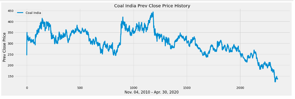
An overview of the dataset

Coal-India Dataset

Cleaning and Visualization of the data

stock.drop(columns=['Symbol','Series','Last','VWAP','Turnover','Trades','Deliverable Volume','%Deliverble'])


#Visualize the Data
plt.figure(figsize=(20,6))
plt.plot(stock['Prev Close'],label = 'Coal India')
plt.title('Coal India Prev Close Price History')
plt.xlabel('Nov. 04, 2010 - Apr. 30, 2020 ')
plt.ylabel('Prev Close Price')
plt.legend(loc='upper left')
plt.show()

We take the Prev. Close Price column because it describes the data best.

Creating Moving Average window

#Creating Simple Moving Average with 30-day Window
Sma30=pd.DataFrame()
Sma30['Prev Close Price']=stock['Prev Close'].rolling(window=30).mean()

#Creating Simple Moving Average with 100-day Window
Sma100=pd.DataFrame()
Sma100['Prev Close Price']=stock['Prev Close'].rolling(window=100).mean()

In the above piece of code, we first created a 30-days MA window (lines 2–3) and then a 100-days MA window (lines 6–7).

Visualizing the results of Moving Average window

Our next step is to visualize the 30-days MA and 100-days MA window and the Prev. Close Price column to compare them.

#Visualize to compare
plt.figure(figsize=(20,6))
plt.plot(stock['Prev Close'],label = 'Coal India')
plt.plot(Sma30['Prev Close Price'],label = 'Sma30')
plt.plot(Sma100['Prev Close Price'],label = 'Sma100')
plt.title('Coal India Prev Close Price History')
plt.xlabel('Nov. 04, 2010 - Apr. 30, 2020 ')
plt.ylabel('Prev Close Price')
plt.legend(loc='upper left')
plt.show()

We can now see the visualization:

Creating a dataframe to store the data

Here, we create a dataframe to store all the required data:

#Creating a new dataframe to store all data
data=pd.DataFrame()
data['stock']=stock['Prev Close']
data['Sma30']=Sma30['Prev Close Price']
data['Sma100']=Sma100['Prev Close Price']

Creating a buy and sell function

Here, we will create two functions buy and sell which will determine the positions of buying and selling shares. It will simply follow the trading criteria as mentioned above.

def buy_sell(data):
  sigPriceBuy=[]
  sigPriceSell=[]
  flag=-1


  for i in range(len(data)):
    if data['Sma30'][i]>data['Sma100'][i]:
      if flag != 1:
        sigPriceBuy.append(data['stock'][i])
        sigPriceSell.append(np.nan)
        flag=1
      else:
        sigPriceBuy.append(np.nan)
        sigPriceSell.append(np.nan)
    elif data['Sma30'][i]<data['Sma100'][i]:
      if flag != 0 :
        sigPriceBuy.append(np.nan)
        sigPriceSell.append(data['stock'][i])
        flag = 0
      else:
        sigPriceBuy.append(np.nan)
        sigPriceSell.append(np.nan)
    else:
      sigPriceBuy.append(np.nan)
      sigPriceSell.append(np.nan)


  return(sigPriceBuy,sigPriceSell)

This will simply create a signal when it is suitable for a trader to buy and sell.

Visualizing the data with signals

Our final work is to visualize where a trader must buy or sell. For this we Store Buy and Sell into a variable. Then we visualize the required plot.

buy_sell = buy_sell(data)
data['Buy_Signal_Price']=buy_sell[0]
data['Sell_Signal_Price']=buy_sell[1]

#Visualize the Data
plt.figure(figsize=(20,6))
plt.plot(stock['Prev Close'],label = 'Coal India',alpha=0.35)
plt.plot(Sma30['Prev Close Price'],label = 'Sma30' ,alpha=0.35)
plt.plot(Sma100['Prev Close Price'],label = 'Sma100' ,alpha=0.35)
plt.scatter(data.index,data['Buy_Signal_Price'],label='Buy',marker='^',color='green')
plt.scatter(data.index,data['Sell_Signal_Price'],label='Sell',marker='v',color='red')
plt.title('Coal India Prev Close Price History Buy and Sell Signals')
plt.xlabel('Nov. 04, 2010 - Apr. 30, 2020 ')
plt.ylabel('Prev Close Price')
plt.legend(loc='upper left')
plt.show()

Output:

The Green signals show where a trader must buy shares of Coal India and the Red signals show where a trader must sell the shares of Coal India so that the trader makes profit in the long run.

Reference : https://medium.com/the-owl/algorithmic-trading-strategies-5c3b9d6ab618

PreviousTrading example NextDOWNLOAD FUNDAMENTALS DATA

Last updated 3 years ago