Portfolio Management
Aug 09, 2019
Portfolio Management Of Multiple Strategies Using Python
In this post we are going to review what a portfolio is, the elements it contains, in addition to reviewing some performance measures, later we will create a simple portfolio with two strategies and several instruments. We will analyze Kelly's method and we will see different combinations that will help us maximize the return and we will compare it with the simple portfolio of equally distributed weights. Finally, we propose a comparison with the classical method of efficient frontier portfolio management. Check out my previous article on Introduction To Portfolio Management which explains all that you need to know about Portfolio Management like techniques, types, derivatives, and much more. In this blog, we will be covering the following topics:
Introduction
Managing a portfolio or Portfolio Management of multiples strategies do not differ much from how to manage a portfolio of assets, only that in this case, the assets are the strategies we have operational. Of course, these strategies handle instruments in which we can be long, short or stay waiting. Obviously, the objective of managing a portfolio of strategies is still to maximize return while minimizing risk. With this simple portfolio, we arrive at the basic question:
How do we distribute capital among the different strategies and instruments in order to maximise the return and minimise the risk?
To have a benchmark with which to compare our optimization we will start from the simple portfolio distributing the same weight for each of its elements. For the optimization of weights in the capital distribution, there are numerous academic studies, each one trying to optimize different parameters. Two of the best known and diametrically opposed methods are:
The efficient frontier proposed by Markowitz in which we try to maximize the return with a certain risk, i.e. it focuses on containing the assigned risk.
On the other hand, there is Kelly's method proposed by John Kelly and Ed Thorpe that tries to maximise the expectation of the log utility of wealth, i.e. maximizing return is the focus.
It is the trader's responsibility to know these and other methods in order to determine which of them best suits his investment style and risk appetite.
Efficient Portfolios
“An efficient portfolio is defined as a portfolio with minimal risk for a given return, or, equivalently, as the portfolio with the highest return for a given level of risk.”
As algorithmic traders, our portfolio is made up of strategies or rules and each of these manages one or more instruments. When we only have one strategy managing one instrument, portfolio management is limited to maximizing return while minimizing risk. This would be the simplest portfolio, but not a simple solution. It is not a simple solution because we have to answer some questions.
Can we achieve the desired return with the instrument we are working with? Are there other instruments that allow us to achieve a higher return with the same risk or less risk with the same return?
On the other hand, if we want to diversify the portfolio and therefore reduce the risk associated with the strategy or instrument, we must build a portfolio with different instruments and ideally different strategies that capture different market regimes. Therefore, in addition to the above questions, we need to answer what weight we assign to each strategy and what weight we give to each instrument within the portfolio to achieve the required objective (Max return vs Min risk).
Portfolio's Elements
Let's define the portfolio's elements which we have some control over them:
Capital: The amount of money we have available to invest or speculate.
Instruments: These are the assets available for inclusion in our portfolio management strategy.
Currency: The currency in which the asset is traded. When we invest in an asset denominated in a foreign currency, we assume the foreign exchange risk.
Volatility: Also called asset risk, indicates the movement of the asset for the period analysed.
Cost: Amount of money needed to buy/sell-short an asset.
Liquidity: It is the capacity of the asset to absorb our operations.
Rules: These are the strategies that try to take advantage of some market regime.
Position weight: The amount of capital we allocate to each asset and/or strategy.
Return: Absolute returns are the return of our portfolio and relative returns are the return of our portfolio compared to a benchmark. When we are not comparing our returns with anybody, absolute return is a good measure, but when we need to compare performances we use the relative return.
Risk or Volatility: This is the (estimated) amount that the portfolio assumes.
Portfolio performance measures
Algorithmic traders have at their disposal a large number of measures to analyze the strategy and/or the portfolio performance. Some of the most used Portfolio performance measures are:
Annualised Returns
Annualised Volatility
Sortino Ratio
Beta
Treynor Ratio
Information Ratio
Skewness
Kurtosis
Maximum Drawdown
Number of Trades
Profit ratio
Holding period
You can find a complete description of these measures in this post. In addition to these individual measures, the pyfolio library implements a fantastic catalogue of performance measures and graphics that are certainly worth learning to use. We will see some of their performance reports through this post.
Building a simple portfolio
To build our example portfolio we are going to use a random time series generated to simulate the return of two strategies over several instruments.
Strategy 1 - The first strategy, that we will call A, is a trend follower system and as it's typical in these strategies, it has a positive bias.
Strategy 2 - The second strategy, that we will call B, is a mean reversion system and as it's typical in these strategies, it has a negative bias.
Role of Bias
The bias or skew is an important concept to characterize the behaviour of the strategy, as it is an indicator of the returns' distribution.
Positive Bias
When we have a positive bias it means that we are having small frequent losses but we capture the infrequent outliers of the distribution. This behaviour is typical of a trend following system since we have frequent false signals with small losses and infrequent large returns, or what is the same, cuts losses quickly and lets the gains run.
Negative Bias
When we have a negative bias it means that we are having small frequent gains and occasional large losses. This behaviour is typical of mean reversion, arbitrage, sell options or similar systems, i.e. we have a system that systematically collects small profits and throws infrequent large losses.
Strategies to be used
In this post, we will work directly with the returns strategies. It is needless to say that any strategy that is considered to be part of the portfolio has had to pass backtesting that offers us an adequate level of uncertainty. Check this post if you need to review the basics of backtesting. What Is Backtesting A Trading Strategy?
About the instruments or assets
Assets are the main elements of a portfolio and their characteristics are decisive for obtaining the determined risk/benefit ratio. Some of the most important characteristics are:
Currency
Volatility
Liquidity
Cost
Commission
Slippage
Correlation (in relation to other assets)
Currency
If our portfolio is denominated in dollars and we buy an instrument on the European stock exchange, we are buying in euros. Therefore, the return on our investment not only depends on the return of the instrument (or strategy) but also depends on the fate of the currency. In the short term, it may be insignificant, but in the long term, it may boost return, reduce it or increase losses.
Volatility
The volatility of the instrument allows us to estimate if we will be able to reach the desired return or if we will be able to contain the required risk. That is to say, if we want to boost the return, we will generally look for more volatile assets and if we want to contain the risk we will look for less volatile assets. It is difficult to raise the return of our strategy to 20% with a treasury bond with an annualized return of 3% (perhaps by increasing the position, leverage or other formulas, but it is difficult). On the other hand, it is difficult to contain the risk of our strategy at 10% if we fill the portfolio of wild penny-stocks with volatilities of more than 300%.
Liquidity
The liquidity of an instrument indicates its capacity to absorb our entry or exit position, logically this is more important for strategies that handle large positions, but the liquidity of a single contract can be critical at certain times (expiration date, moments of panic, etc.).
Cost
The cost of the asset allows us to know the position and the weight that the asset will have within our portfolio. Let's suppose that we have a strategy that exploits a characteristic of the gold price. We can invest in gold in multiple ways, among them we can buy Gold futures contracts, e-mini Gold and Micro Gold, we have available Options, ETF, etc. each with a cost, volatility, commissions, slippage, etc.
Commission and Slippage
Commissions and slippage undermine the return on our portfolio and should be studied in depth. The slippage is closely related to the bid-ask price.
Correlation
Finally, when we are analyzing different instruments to include in our portfolio of strategies it is necessary to take into account the correlation with possible candidates. For example, if our portfolio strategy is exploiting a trend following system with an e-mini gold contract, it would not make much sense from a diversification point of view to include the future of silver which usually has a high correlation with gold. Ideally, we will look for low correlation assets to exploit the same strategy.
Importing the libraries and data
Multiple Strategies
Strategy A - Trend following system - Instrument 1
Here we have simulated the return of a trend following strategy and forced it to have a Sharpe Ratio of 0.5 and skewness of 1. In [ ]:
Out [ ]

Strategy A - Trend following system - Instrument 2
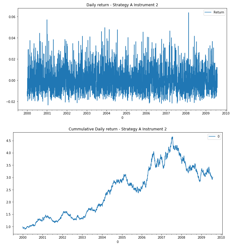
Here we have simulated the return of a trend following strategy and forced it to have a Sharpe Ratio of 1 and skewness of 1. In [ ]:
Out[ ]:
Strategy A - Trend following system - Instrument 3
Here we have simulated the return of a trend following strategy and forced it to have a Sharpe Ratio of 1 and skewness of 1.
Although it has the same characteristics as the previous one, the volatility is different and allows us to evaluate its contribution within the portfolio.
In [ ]:
Out[ ]:

Strategy B - Mean reversion system - Instrument 1
Here we have simulated the return of a mean reversion strategy and forced it to have a Sharpe Ratio of 0.5 and skewness of -1.
In [ ]:
Out[ ]:

Strategy B - Mean reversion system - Instrument 2
Here we have simulated the return of a mean reversion strategy and forced it to have a Sharpe Ratio of 1 and skewness of -1.
In [ ]:
Out[ ]:

Portfolio Strategies
Portfolio with strategies A and B - 5 Instruments
In order to facilitate the analysis, we create a dataframe with all the returns we have.
In [ ]:
Out[ ]:

In [ ]
Out[ ]:

Portfolio with the strategy A - 3 Instruments
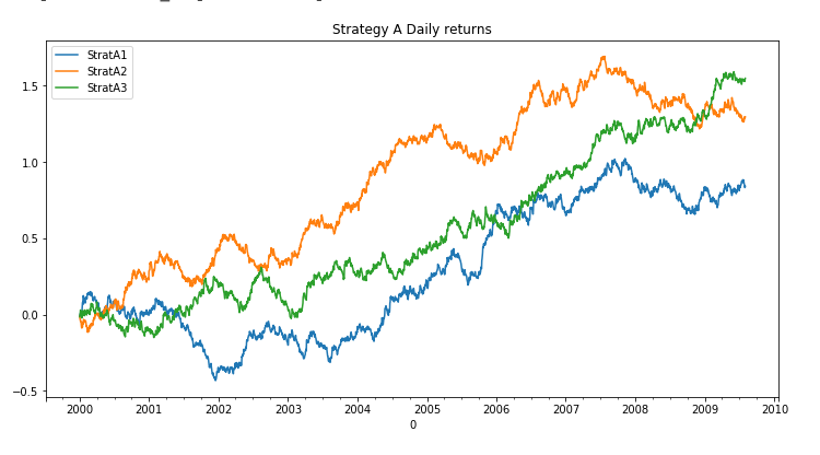
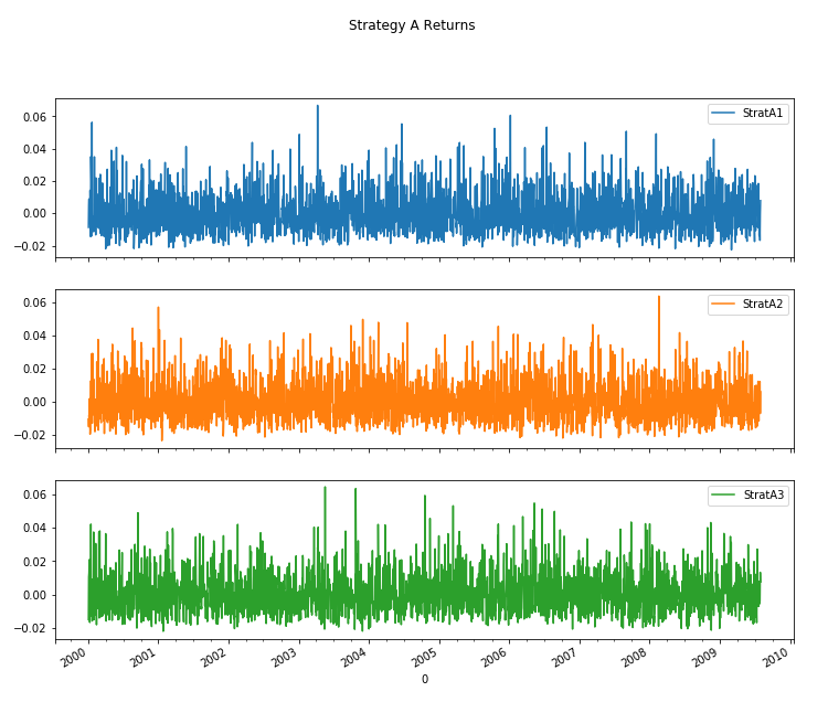
In order to facilitate the analysis, we create a dataframe with all the strategy A returns.
In [ ]:
Out[ ]:
In [ ]
Out[ ]:
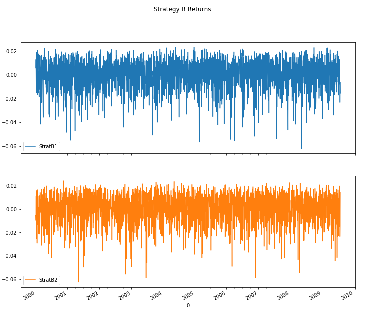
Portfolio with strategy B - 2 Instruments
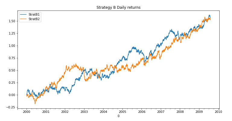
In order to facilitate the analysis, we create a dataframe with all the strategy B returns.
In [ ]:
Out[ ]:
In[ ]:
Out[ ]:
Basic Analysis
Some basic functions to characterize individually the returns.
In [ ]:
Out[ ]:
StratA1
StratA2
StratA3
StratB1
StratB2
count
2500.000000
2500.000000
2500.000000
2500.000000
2500.000000
mean
0.000336
0.000518
0.000619
0.000625
0.000613
std
0.012382
0.012449
0.012265
0.012167
0.012487
min
-0.022628
-0.023483
-0.022159
-0.061927
-0.062419
25%
-0.008736
-0.008848
-0.008323
-0.006073
-0.006649
50%
-0.001367
-0.001429
-0.001100
0.002460
0.002505
75%
0.007027
0.007482
0.007427
0.009481
0.009931
max
0.066684
0.063726
0.064527
0.023033
0.024209
Return distribution
In [ ]:
Out[ ]:
In [ ]:
Out[ ]:
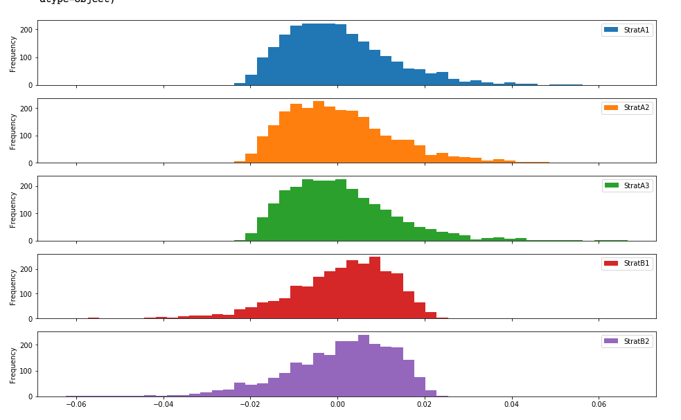
Here we can see the distribution of returns for each of the strategies we have in hand.
In [ ]:
Out[ ]:
As we commented before, correlation is vital to know when asset or strategy returns go hand in hand in future luck. To benefit from diversification, the correlation must be 'low'.
We can calculate the correlation between the returns of the strategies with the whole series
In [ ]:
Out[ ]:
StratA1
StratA2
StratA3
StratB1
StratB2
StratA1
1.000000
0.002856
-0.025571
0.030596
-0.002940
StratA2
0.002856
1.000000
0.035310
-0.025093
0.020062
StratA3
-0.025571
0.035310
1.000000
0.026725
0.020929
StratB1
0.030596
-0.025093
0.026725
1.000000
-0.011878
StratB2
-0.002940
0.020062
0.020929
-0.011878
1.000000
Or analyze the correlation based on the time horizon we have as an investment
In [ ]:
Out[ ]:
StratA1
StratA2
StratA3
StratB1
StratB2
StratA1
1.000000
-0.251070
-0.068042
0.199785
0.128537
StratA2
-0.251070
1.000000
-0.038942
-0.086718
-0.033532
StratA3
-0.068042
-0.038942
1.000000
-0.091949
0.063135
StratB1
0.199785
-0.086718
-0.091949
1.000000
-0.267339
StratB2
0.128537
-0.033532
0.063135
-0.267339
1.000000
The above analyses give us a snapshot at a given time for a given horizon, but the reality is that the correlation varies over time and knowing this allows us to make better estimates.
For example, we can see that the correlation is different if we consider a year:
In [ ]:
Out[ ]:

A quarter's correlation is greater than the annual correlation. In[ ]:
Out[ ]:

If we reduce the horizon to two weeks, we see that the correlation is quite high. Therefore, we see that the correlation is closely related to the analysis horizon.
In [ ]:
Out[ ]:

Basic performance analysis
Although logically all performance indicators can be calculated by hand, it is worth knowing the pyfolio library offers us an immense amount of information about the performance of our strategy.
In [ ]:
Start date
2000-01-03
End date
2009-07-31
Total months
119
Backtest
Annual return
6.8%
Cumulative returns
91.5%
Annual volatility
19.7%
Sharpe ratio
0.43
Calmar ratio
0.15
Stability
0.68
Max drawdown
-46.0%
Omega ratio
1.07
Sortino ratio
0.72
Skew
0.98
Kurtosis
1.45
Tail ratio
1.44
Daily value at risk
-2.4%
Worst drawdown periods
Net drawdown in %
Peak date
Valley date
Recovery date
Duration
0
45.99
2000-02-25
2001-12-17
2005-01-21
1281
1
31.85
2007-11-08
2008-11-07
NaT
NaN
2
21.48
2005-05-20
2005-08-04
2005-10-21
111
3
14.81
2006-08-04
2007-01-02
2007-03-19
162
4
13.67
2006-01-09
2006-06-19
2006-07-17
136

To understand the information in the report, you can read more in this post: Performance & risk metrics optimization
Equal weighted portfolio
As you can suppose, the problem we are dealing with is knowing how to distribute the available capital between each of the portfolio strategies that have passed the mandatory robust backtesting.
To know if we are doing well, we need something to compare ourselves with, the benchmark, and it must have characteristics similar to what we want to compare.
For example, the trend following system should be compared with a strategy of buying and holding a portfolio with the same assets.
Here we are going to create a portfolio whose weights are identical for each of the instruments, not differentiate the type of strategy. It serves as a basis for comparing the balance of weights that we will be testing.
In [ ]:
Once the total return of the equally distributed portfolio has been computed, we generate the performance report.
In [ ]:
Start date
2000-01-03
End date
2009-07-31
Total months
119
Backtest
Annual return
14.2%
Cumulative returns
272.8%
Annual volatility
8.9%
Sharpe ratio
1.54
Calmar ratio
1.34
Stability
0.97
Max drawdown
-10.6%
Omega ratio
1.28
Sortino ratio
2.39
Skew
0.10
Kurtosis
0.06
Tail ratio
1.18
Daily value at risk
-1.1%
Worst drawdown periods
Net drawdown in %
Peak date
Valley date
Recovery date
Duration
0
10.56
2002-09-23
2003-02-19
2003-04-17
149
1
9.39
2006-01-18
2006-03-07
2006-04-05
56
2
9.13
2001-03-26
2001-08-21
2001-12-20
194
3
8.79
2007-07-25
2008-04-24
2008-12-25
372
4
7.41
2002-01-23
2002-04-19
2002-06-06
97

Portfolio weights optimized with Kelly criterion
Kelly's criterion is one of the methods available to estimate the weights of our portfolio and maximize the benefit with minimum risk for the analyzed portfolio.
First, we get the number of stocks inside the portfolio.In [ ]:
Out[ ]:
In [ ]:
Out[ ]:
The portfolio returns are based on the daily return multiplied by the weight for each asset.In [ ]:
Out[ ]:
Kelly Criterion
The final portfolio value or the utility of the portfolio can be computed using the logarithmic summation of the daily portfolio returns.In [ ]:
Out[ ]:
The output tells us that the final_portfolio_value is an expression and is concave in nature and its value is unknown
The objective of this example is to maximise the Kelly criterion. To do this, you can create a parameter called 'objective' and assign the maximisation condition to it. The Maximize function of the cvxpy library is used for this purpose.In [ ]:
Out[ ]:
The output tells us that the objective is a Maximize function over the expression. The expression is concave in nature and its value is unknown
Before you solve the objective, you need to remember that there are certain constraints on the weights of the portfolio.
The weights should positive, as you are considering to use a strategy or not.
The sum of weights should be less than or equal to 1, as you are not considering leveraging.
In [ ]:
Out[ ]:
Here the constraints specify that the first one is an inequality constraint and its value is a constant zero. While the second is an equality constraint between an affine expression whose value is equal to a constant non-negative value
Now, you can combine both the objective and the constraints to create a problem statement. You can do this by using the Problem class of the cvxpy library, as shown below.In [ ]:
Out[ ]:
Here the output describes the entire problem including all the previously described expression into a one single statement
You can use the solve method of the problem class to get the best weight combination as shown below:In [ ]:
Out[ ]
These are the optimal weights according to Kelly's criterion, as we can see the first two strategies have such a small weight that we discard them and simplified, we can say that the remaining three have a similar weight.In [ ]:
Start date
2000-01-03
End date
2009-07-31
Total months
119
Backtest
Annual return
16.1%
Cumulative returns
340.7%
Annual volatility
11.5%
Sharpe ratio
1.36
Calmar ratio
0.96
Stability
0.96
Max drawdown
-16.8%
Omega ratio
1.24
Sortino ratio
2.00
Skew
-0.20
Kurtosis
0.53
Tail ratio
1.05
Daily value at risk
-1.4%
Worst drawdown periods
Net drawdown in %
Peak date
Valley date
Recovery date
Duration
0
16.83
2005-11-07
2006-03-07
2006-05-30
147
1
13.79
2002-08-13
2003-02-19
2003-05-23
204
2
12.97
2000-01-28
2000-06-09
2001-03-05
287
3
10.05
2002-01-23
2002-04-19
2002-06-17
104
4
9.59
2003-09-02
2003-10-16
2004-05-06
178

If we compare it with the initial portfolio with the equally distributed weights, we see that Kelly's optimization has improved the annualized return and the cumulative one, but in contrast, we have decreased the SR and increased the volatility.
Kelly Strategy A
We are going to repeat the same exercise for the two strategies in an individualized way, in this way we want to know which weights we should assign to each one of the assets of a strategy.
In [ ]:
Out[ ]
Start date
2000-01-03
End date
2009-07-31
Total months
119
Backtest
Annual return
14.8%
Cumulative returns
293.1%
Annual volatility
17.0%
Sharpe ratio
0.90
Calmar ratio
0.58
Stability
0.94
Max drawdown
-25.4%
Omega ratio
1.16
Sortino ratio
1.55
Skew
0.98
Kurtosis
1.54
Tail ratio
1.50
Daily value at risk
-2.1%
Worst drawdown periods
Net drawdown in %
Peak date
Valley date
Recovery date
Duration
0
25.36
2002-08-13
2003-01-17
2003-08-26
271
1
17.16
2001-12-12
2002-04-22
2002-08-01
167
2
16.56
2000-03-31
2000-08-29
2001-06-07
310
3
15.45
2005-11-07
2006-03-06
2006-05-08
131
4
13.20
2004-05-13
2004-07-16
2004-10-19
114
Start date
2000-01-03
End date
2009-07-31
Total months
119
Backtest
Annual return
7.5%
Cumulative returns
104.1%
Annual volatility
6.8%
Sharpe ratio
1.09
Calmar ratio
0.57
Stability
0.93
Max drawdown
-13.1%
Omega ratio
1.19
Sortino ratio
1.78
Skew
0.58
Kurtosis
0.51
Tail ratio
1.30
Daily value at risk
-0.8%
Worst drawdown periods
Net drawdown in %
Peak date
Valley date
Recovery date
Duration
0
13.09
2007-09-13
2008-11-11
NaT
NaN
1
7.71
2002-09-23
2003-02-19
2003-04-17
149
2
7.48
2001-03-28
2001-08-21
2002-08-13
360
3
7.36
2005-05-23
2005-08-04
2005-11-04
120
4
4.72
2003-05-20
2003-08-05
2003-09-30
96

Again we observe the same as with the complete portfolio, with Kelly's optimization we increase returns, but in contrast, we have decreased the SR and increased the volatility.
Kelly Strategy B
The same for assets in strategy B
In [ ]:
Out[ ]:
Start date
2000-01-03
End date
2009-07-31
Total months
119
Backtest
Annual return
15.8%
Cumulative returns
327.8%
Annual volatility
13.8%
Sharpe ratio
1.13
Calmar ratio
0.87
Stability
0.96
Max drawdown
-18.2%
Omega ratio
1.20
Sortino ratio
1.55
Skew
-0.68
Kurtosis
0.68
Tail ratio
0.84
Daily value at risk
-1.7%
Worst drawdown periods
Net drawdown in %
Peak date
Valley date
Recovery date
Duration
0
18.17
2005-12-27
2006-03-07
2006-06-09
119
1
16.13
2002-12-18
2003-10-14
2004-08-03
425
2
14.76
2000-01-28
2000-06-09
2000-11-16
210
3
11.07
2002-01-29
2002-04-01
2002-05-15
77
4
10.15
2006-11-08
2006-12-13
2007-01-25
57
Start date
2000-01-03
End date
2009-07-31
Total months
119
Backtest
Annual return
6.3%
Cumulative returns
82.9%
Annual volatility
5.5%
Sharpe ratio
1.13
Calmar ratio
0.84
Stability
0.96
Max drawdown
-7.5%
Omega ratio
1.20
Sortino ratio
1.55
Skew
-0.67
Kurtosis
0.61
Tail ratio
0.85
Daily value at risk
-0.7%
Worst drawdown periods
Net drawdown in %
Peak date
Valley date
Recovery date
Duration
0
7.46
2005-12-27
2006-03-07
2006-05-31
112
1
6.74
2002-12-18
2003-10-14
2004-05-27
377
2
6.21
2000-01-28
2000-06-09
2000-11-16
210
3
4.56
2002-01-29
2002-04-01
2002-05-15
77
4
4.39
2006-11-08
2006-12-13
2007-01-25
57

Again we observe the same as with the complete portfolio, with Kelly's optimization we increase returns, but in contrast, we have decreased the SR and increased the volatility.
Kelly Strategy A & B
Now that we have the optimized weights for each strategy independently, we are going to optimize the weights that we will assign to each strategy.
In [ ]:
Out[ ]:
Start date
2000-01-03
End date
2009-07-31
Total months
119
Backtest
Annual return
16.0%
Cumulative returns
337.7%
Annual volatility
11.0%
Sharpe ratio
1.41
Calmar ratio
1.03
Stability
0.97
Max drawdown
-15.6%
Omega ratio
1.25
Sortino ratio
2.04
Skew
-0.32
Kurtosis
0.49
Tail ratio
1.00
Daily value at risk
-1.3%
Worst drawdown periods
Net drawdown in %
Peak date
Valley date
Recovery date
Duration
0
15.64
2005-11-07
2006-03-07
2006-05-24
143
1
12.36
2000-01-28
2000-06-09
2000-12-25
237
2
12.34
2002-08-13
2003-02-19
2003-04-21
180
3
9.76
2002-01-23
2002-04-01
2002-06-18
105
4
8.76
2003-09-02
2003-10-16
2004-03-05
134
Start date
2000-01-03
End date
2009-07-31
Total months
119
Backtest
Annual return
6.3%
Cumulative returns
82.6%
Annual volatility
4.4%
Sharpe ratio
1.39
Calmar ratio
0.96
Stability
0.97
Max drawdown
-6.5%
Omega ratio
1.25
Sortino ratio
2.19
Skew
0.29
Kurtosis
0.66
Tail ratio
1.20
Daily value at risk
-0.5%
Worst drawdown periods
Net drawdown in %
Peak date
Valley date
Recovery date
Duration
0
6.55
2002-08-13
2003-02-19
2003-05-19
200
1
6.43
2005-11-07
2006-03-07
2006-05-11
134
2
4.57
2002-01-23
2002-04-19
2002-06-26
111
3
4.49
2000-01-28
2000-06-09
2001-03-01
285
4
3.57
2007-09-07
2007-12-17
2008-02-28
125

So what we now have are two strategies with several instruments, we have optimized the weight of the instruments for each strategy independently. We have re-applied the optimization method to the return of each of the portfolios of optimized strategies, giving us the final weight of the portfolio.
We can see it more clearly in a table.
Capital divided by strategy type according to the last optimization.
The capital assigned to each strategy is divided by the optimal weights.
The Efficient Frontier: Markowitz Portfolio Optimization
We can repeat the same exercise using the efficient frontier proposed by Markowitz. His method is based on maximizing the Sharpe ratio of a portfolio given the mean, standard deviation and correlations. However, since the method assumes the same volatility and return for each strategy, the weights it offers are more extreme than Kelly's.
Read the following post and webinar for a complete explanation Multi-Strategy Portfolios: Combining Quantitative Strategies Effectively
In [ ]:
In [ ]:
In [ ]:
In [ ]:
In [ ]:
In [ ]:
In [ ]:
In [ ]:
In [ ]:
In [ ]:
In [ ]:
In [ ]:
In [ ]:
In [ ]:
In [ ]:
In [ ]:
In [ ]:
In [ ]:
In [ ]:
In [ ]:
In [ ]:
Conclusion
The optimization of strategy portfolios is not far from the optimization that we will make to a portfolio of instruments since we are working with returns.
Strategies and instruments must be characterized in order to know when they add value to the portfolio or not (although the strategy offers interesting returns, it may not add value to the portfolio as a whole or even increase the risk).
Here we have seen two methods that offer different results basically because their assumptions are different, there are other methods with different results, this detail is important depending on the type of portfolio we are trying to optimize. If you are a trader who faces some of the inevitable questions on a day to day basis like - Where should I invest? How much risk to take? How to reduce portfolio volatility? - be sure to check our previous webinar on Quantitative Portfolio Management Strategies. We hope this blog has been helpful to you. You could also check out all our blogs on Portfolio Management here. Please feel free to share your comments below.
Disclaimer: All investments and trading in the stock market involve risk. Any decisions to place trades in the financial markets, including trading in stock or options or other financial instruments is a personal decision that should only be made after thorough research, including a personal risk and financial assessment and the engagement of professional assistance to the extent you believe necessary. The trading strategies or related information mentioned in this article is for informational purposes only. Files in the download: Blog Python Code and 7 data files
Last updated