Stock Market Analysis
Aug 06, 2019
Stock Market Data And Analysis In Python
In this article, you will learn to get the stock market data such as price, volume and fundamental data using python packages and how to analyze it.
In backtesting your strategies or analyzing the performance, one of the first hurdles faced is getting the right stock market data and in the right format, isn't it? Don't worry.
After reading this, you will be able to:
Fetch the open, high, low, close, and volume data.
Get data at a custom frequency such as 1 minute, 7 minutes or 2 hours
Perform analysis of your portfolio
Get the earnings data, balance sheet data, cash flow statements and various key ratios such as price to earnings (PE) and price to book value (PB)
Get the futures and options data for Indian stock market
Generally, web sources are quite unstable and therefore, you will learn to get the stock market data from multiple web sources. For easy navigation, this article is divided as below.
Price Volume Daily Data
Yahoo Finance
One of the first sources from which you can get daily price-volume stock market data is Yahoo finance. You can use pandas_datareader or yfinance module to get the data.
In [ ]:
In [22]:
Out[22]:
In [7]:
Out[7]:
Date
High
Low
Open
Close
Volume
Adj Close
1997-05-15
2.500000
1.927083
2.437500
1.958333
72156000.0
1.958333
1997-05-16
1.979167
1.708333
1.968750
1.729167
14700000.0
1.729167
1997-05-19
1.770833
1.625000
1.760417
1.708333
6106800.0
1.708333
1997-05-20
1.750000
1.635417
1.729167
1.635417
5467200.0
1.635417
1997-05-21
1.645833
1.375000
1.635417
1.427083
18853200.0
1.427083
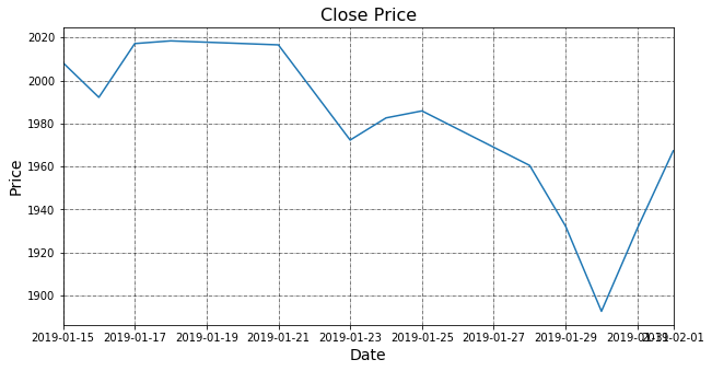
To visualize the adjusted close price data, you can use the matplotlib library and plot method as shown below.
In [9]:

Let us improve the plot by resizing, giving appropriate labels and adding grid lines for better readability.
In [10]:

Advantages
Adjusted close price stock market data is available
Most recent stock market data is available
Doesn't require API key to fetch the stock market data
Disadvantages
It is not a stable source to fetch the stock market data
If the stock market data fetching fails from yahoo finance using the pandas_datareaderthen you can use yfinance package to fetch the data.
Quandl
Quandl has many data sources to get different types of data. However, some are free and some are paid. Wiki is the free data source of Quandl to get the data of the end of the day prices of 3000+ US equities. It is curated by Quandl community and also provides information about the dividends and split. To get the stock market data, you need to first install the quandl module if it is not already installed using the pip command as shown below.
In [ ]:
You need to get your own API Key from quandl to get the stock market data using the below code. If you are facing issue in getting the API key then you can refer to this link.
After you get your key, assign the variable QUANDLAPIKEYQUANDLAPIKEY with that key. Then set the start date, end date and the ticker of the asset whose stock market data you want to fetch.
The quandl get method takes this stock market data as input and returns the open, high, low, close, volume, adjusted values and other information.
In [1]:
Out[1]:
Date
Open
High
Low
Close
Volume
Ex-Dividend
Split Ratio
Adj. Open
Adj. High
Adj. Low
Adj. Close
Adj. Volume
1997-05-16
22.38
23.75
20.50
20.75
1225000.0
0.0
1.0
1.865000
1.979167
1.708333
1.729167
14700000.0
1997-05-19
20.50
21.25
19.50
20.50
508900.0
0.0
1.0
1.708333
1.770833
1.625000
1.708333
6106800.0
1997-05-20
20.75
21.00
19.63
19.63
455600.0
0.0
1.0
1.729167
1.750000
1.635833
1.635833
5467200.0
1997-05-21
19.25
19.75
16.50
17.13
1571100.0
0.0
1.0
1.604167
1.645833
1.375000
1.427500
18853200.0
1997-05-22
17.25
17.38
15.75
16.75
981400.0
0.0
1.0
1.437500
1.448333
1.312500
1.395833
11776800.0
In [3]:

Get stock market data for multiple tickers
To get the stock market data of multiple stock tickers, you can create a list of tickers and call the quandl get method for each stock ticker.[1]
For simplicity, I have created a dataframe data to store the adjusted close price of the stocks.
In [4]:
Out[4]:
Date
AAPL
IBM
MSFT
WMT
1990-01-02
1.118093
14.138144
0.410278
4.054211
1990-01-03
1.125597
14.263656
0.412590
4.054211
1990-01-04
1.129499
14.426678
0.424702
4.033561
1990-01-05
1.133101
14.390611
0.414300
3.990541
1990-01-08
1.140605
14.480057
0.420680
4.043886
In [5]:

Advantages
It is free of cost
Has split and dividend-adjusted stock market data
Disadvantages
Only available till 27-March-2018
Intraday Data
Alpha Vantage
Alpha vantage is used to get the minute level stock market data. You need to signup on alpha vantage to get the free API key.
In [ ]:
Assign the ALPHA_VANTAGE_API_KEY, with your API Key in the below code.
In [12]:
Out[12]:
This gives information about the stock market data which is returned. The information includes the type of data returned such as open, high, low and close, the symbol or ticker of the stock, last refresh time of the data, frequency of the stock market data and the time zone.
In [13]:
Out[13]:
Date
Open
High
Low
Close
Volume
2019-07-26 09:31:00
1228.2300
1232.49
1228.0000
1230.7898
407037.0
2019-07-26 09:32:00
1230.9200
1235.13
1230.4301
1233.0000
111929.0
2019-07-26 09:33:00
1233.0000
1237.90
1232.7500
1237.9000
86564.0
2019-07-26 09:34:00
1237.4449
1241.90
1237.0000
1241.9000
105884.0
2019-07-26 09:35:00
1241.9399
1244.49
1241.3500
1243.1300
74444.0
In [19]:

Get data at a custom frequency
During strategy modelling, you are required to work with a custom frequency of stock market data such as 7 minutes or 35 minutes. This custom frequency candles are not provided by data vendors or web sources. In this case, you can use the pandas resample method to convert the stock market data to the frequency of your choice. The implementation of these is shown below where a 1-minute frequency data is converted to 10-minute frequency data.
The first step is to define the dictionary with the conversion logic. For example, to get the open value the first value will be used, to get the high value the maximum value will be used and so on.
In [ ]:
Convert the index to datetime timestamp as by default string is returned. Then call the resample method with the frequency such as
10T for 10 minutes,
D for 1 day and
M for 1 month
In [130]:
Out[130]:
Date
Open
High
Low
Close
Volume
2019-07-17 09:30:00
1150.9200
1155.5500
1150.510
1154.28
82911.0
2019-07-17 09:40:00
1154.2950
1157.8400
1154.295
1157.76
35549.0
2019-07-17 09:50:00
1157.4250
1158.4399
1155.670
1155.67
30371.0
2019-07-17 10:00:00
1155.4700
1156.0200
1153.090
1153.09
21445.0
2019-07-17 10:10:00
1153.0194
1153.4200
1151.000
1152.29
31073.0
yfinance
yfinance is another module which can be used to fetch the minute level stock market data. It returns the stock market data for the last 7 days.
In [ ]:
The yfinance module has the download method which can be used to download the stock market data. It takes the following parameters:
ticker: The name of the tickers you want the data for. If you want data for multiple tickers then separate them by spaceperiod: The number of days/month of data required. The valid frequencies are 1d, 5d, 1mo, 3mo, 6mo, 1y, 2y, 5y, 10y, ytd, maxinterval: The frequency of data. The valid intervals are 1m, 2m, 5m, 15m, 30m, 60m, 90m, 1h, 1d, 5d, 1wk, 1mo, 3mo
The below code fetches the stock market data for MSFT for the past 5 days of 1-minute frequency.
In [133]:
Out[133]:
Datetime
Open
High
Low
Close
Adj Close
Volume
2019-07-17 09:30:00-04:00
137.70
137.75
137.23
137.33
137.33
645676
2019-07-17 09:31:00-04:00
137.33
137.43
137.22
137.40
137.40
112675
2019-07-17 09:32:00-04:00
137.39
137.40
137.18
137.29
137.29
73906
2019-07-17 09:33:00-04:00
137.44
137.58
137.39
137.42
137.42
127492
2019-07-17 09:34:00-04:00
137.44
137.52
137.43
137.45
137.45
56630
Stocks Fundamental Data
We have used yfinance to get the fundamental data. The first step is to set the ticker and then call the appropriate properties to get the right stock market data.
In [ ]:
In [ ]:
Key Ratios
You can fetch the latest price to book ratio and price to earnings ratio as shown below.
In [ ]:
Revenues
In [134]:

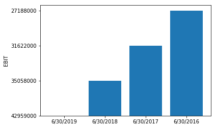
Earnings Before Interest and Taxes
In [135]:
Balance sheet, cash flows and other information
In [ ]:
Futures and Options (F&O) Data for Indian Equities
NSEpy
The nsepy package is used to get the stock market data for the futures and options for Indian stocks and indices.
Futures Data
In [15]:
Out[15]:
Date
Symbol
Expiry
Open
High
Low
Close
Last
Settle Price
Number of Contracts
Turnover
Open Interest
Change in OI
Underlying
2019-01-15
HDFC
2019-02-28
1986.70
2011.00
1982.95
2008.25
2006.20
2008.25
4810
4.796817e+09
2537500
2299500
1992.15
2019-01-16
HDFC
2019-02-28
2002.10
2010.15
1985.20
1992.15
1991.30
1992.15
2656
2.655748e+09
3783500
1246000
1975.00
2019-01-17
HDFC
2019-02-28
2003.60
2019.05
1991.60
2017.15
2013.00
2017.15
3993
4.008667e+09
5545000
1761500
NaN
2019-01-18
HDFC
2019-02-28
2018.55
2025.75
2005.00
2018.40
2017.25
2018.40
481
4.845300e+08
5637000
92000
2006.85
2019-01-21
HDFC
2019-02-28
2011.25
2031.10
1998.00
2016.55
2016.60
2016.55
1489
1.505249e+09
6258000
621000
2004.45
In [20]:
Options Data
In [17]:
Out[17]:
Date
Symbol
Expiry
Option Type
Strike Price
Open
High
Low
Close
Last
Settle Price
Number of Contracts
Turnover
Premium Turnover
Open Interest
Change in OI
Underlying
2019-01-15
HDFC
2019-02-28
CE
2000.0
52.70
56.00
52.70
56.0
56.0
56.0
3
3081000.0
81000.0
10000
1000
1992.15
2019-01-16
HDFC
2019-02-28
CE
2000.0
55.00
55.00
49.00
49.0
49.0
49.0
14
14358000.0
358000.0
11000
1000
1975.00
2019-01-17
HDFC
2019-02-28
CE
2000.0
59.15
64.65
51.00
61.9
61.9
61.9
27
27750000.0
750000.0
18500
7500
NaN
2019-01-18
HDFC
2019-02-28
CE
2000.0
63.00
63.00
60.00
60.0
60.0
60.0
7
7212000.0
212000.0
18500
0
2006.85
2019-01-21
HDFC
2019-02-28
CE
2000.0
62.05
69.00
62.05
62.9
62.9
62.9
6
6198000.0
198000.0
20000
1500
2004.45
In [21]:

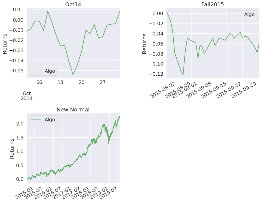
Visualization and Analysis
After you have the stock market data, the next step is to create trading strategies and analyze the performance. I have created a simple buy and hold strategy for illustration purpose with four stocks namely Apple, Amazon, Microsoft and Walmart. To analyze the performance, you can use the pyfolio tear sheet as shown below.
In [ ]:
In [ ]:
In [16]:
Out[16]:
In [21]:
Start date
2014-07-29
End date
2019-07-25
Total months
59
Backtest
Annual return
26.6%
Cumulative returns
224.4%
Annual volatility
18.2%
Sharpe ratio
1.39
Calmar ratio
1.11
Stability
0.96
Max drawdown
-24.1%
Omega ratio
1.28
Sortino ratio
2.07
Skew
0.15
Kurtosis
4.25
Tail ratio
0.94
Daily value at risk
-2.2%
Worst drawdown periods
Net drawdown in %
Peak date
Valley date
Recovery date
Duration
0
24.08
2018-10-01
2018-12-24
2019-04-17
143
1
13.15
2015-07-30
2015-08-25
2015-10-23
62
2
13.12
2015-12-07
2016-02-09
2016-04-13
93
3
9.65
2019-05-03
2019-06-03
2019-06-18
33
4
8.46
2018-03-12
2018-04-02
2018-05-10
44
Stress Events
mean
min
max
Oct14
0.04%
-1.68%
2.17%
Fall2015
-0.17%
-4.67%
5.35%
New Normal
0.10%
-4.67%
7.17%


I hope you can use the Python codes to fetch the stock market data of your favourites stocks, build the strategies and analyze it. I would appreciate if you could share your thoughts and your comments below. Python is quite essential to understand data structures, data analysis, dealing with financial data, and for generating trading signals. For traders and quants who want to learn and use Python in trading, this bundle of courses is just perfect. Disclaimer: All investments and trading in the stock market involve risk. Any decisions to place trades in the financial markets, including trading in stock or options or other financial instruments is a personal decision that should only be made after thorough research, including a personal risk and financial assessment and the engagement of professional assistance to the extent you believe necessary. The trading strategies or related information mentioned in this article is for informational purposes only.
Reference : https://blog.quantinsti.com/stock-market-data-analysis-python/
Last updated